


 ,
,
发表评论

扫码加微信:-)
扫码加微信:-)
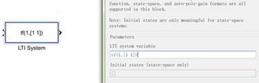
Analysis Interface for Linear SystemsModeling of Linear SystemsSimulink提供了各种用来对线性系统建模的工具诸如:转移函数,态空间和zpk模块等.这些模块既有连续的也由离散的.同时还有线性时变对象(LTI),诸如tf对象,ss对象和zpk对象. G=tf(n,d) %n,d分别代表多项式分子系数 和 分母系数 G=ss(A,B,C,D);%ABCD为态空间描述矩阵 G=zpk(z,p,K) 采样数据系统同样可以使用相同的方法表达,采样间隔时间T=G.Ts 不带有延时的LTI对象可以用LTI系统模块(在控制系统工具箱),直接填写LTI变量即可,如果采用ss模型则还可以填写初始态参数.
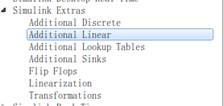
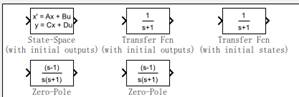
带有初始条件的线性系统可以同通过Simulink Extras->Additional Linear中找到
Example 4.7 Consider the transfer function model >> %转移函数的一种声明方式 >> s=tf('s'); >> G=(s^2+5)/(s^2*(s+1)^2*(s+2)^2+9) G = s^2 + 5 ----------------------------------------- s^6 + 6 s^5 + 13 s^4 + 12 s^3 + 4 s^2 + 9 Continuous-time transfer function. Example
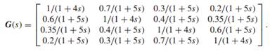
4.8 Transfer function matrices of multivariable systems can also be
represented by
对于上面的多变量系统使用低阶的模块处理非常困难,然而使用LTI则该系统则比较容易建模. h1=tf(1,[4 1]); h2=tf(1,[5 1]); %其成员都是h1和h2的倍数; h11=h1; h12=0.7*h2; h13=0.5*h2; h14=0.2*h2; h21=0.6*h2; h22=h1; h23=0.4*h2; h24=0.35*h2; h31=h24; h32=h23; h33=h1; h34=h21; h41=h14; h42=h13; h43=h12; h44=h1; G=[h11,h12,h13,h14; h21,h22,h23,h24; h31,h32,h33,h34; h41,h42,h43,h44]; Example 4.9 Consider the discrete state space model given by
其采样间隔为T=0.1s,LTI中的变量G可以如下声明: F=[0,-2,-2,-1.1; 0.5,1.8,0.8,0.5; 0.5,0.8,1.8,0.5;
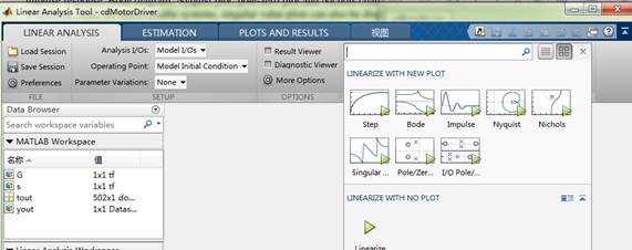
-0.5,-0.8,-0.7,0.4]; Analysis Interface for Linear SystemsMatlab提供了很多分析工具,例如bode(G)用来分析系统的伯特图.nyquist(G)和nichols(G)用来绘制奈奎斯特图和尼古拉斯图.step(G)和impulse(G)用来画越截图和脉冲图
Analysis->Control Desgin ->Linear Analysis
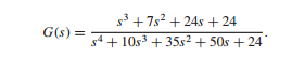
4.6 Simulation of Continuous Nonlinear Stochastic Systems(连续非线性随机系统的仿真)在第三章曾经提及对于由白噪音驱动的连续系统,随机数生成器不能直接使用.第三章的处理也仅仅是在线性系统中使用.利用文献中介绍的非线性随机性处理方法非常难以扩展. 4.6.1 Simulation of Random Signals in Simulink(随机信号的仿真)在Source群组中的Band-Limited White Noise(带宽限定白噪声)模块可以用来模拟指定强度的白噪音输入.十几场该模块扮演了1/sqrt(Δt)*Rand()的脚色. Example 4.10 Consider again the system model shown in Example 3.36.
Approximate simulation methods can be used, and the Simulink model is
constructed in Fig. 4.61(a). Selecting 考虑3.36模型
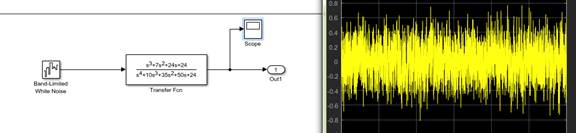
对模型参数进行设定,固定补偿为0.1s ,计算时间为3000s.计算结果如下:
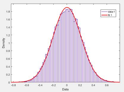
通过统计算法画出信号的概率密度函数
4.6.2 Statistical Analysis of Simulation Results(仿真结果的统计分析)
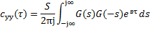
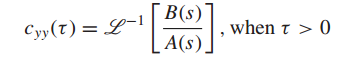
Cyy是由高斯白噪声驱动输出信号的自动相关函数,是一个双边反拉普拉斯变换.其中S是白噪声的功率谱密度.根据谱分解理论,G(s)G(-s)可以分解为:
这其中A(s)是G(s)G(-s)的分母,其极点在s平面的左侧,数学上A(s)被记为D(s)_,D(s)和N(s)则是多项式G(s)的分母和分子.有:
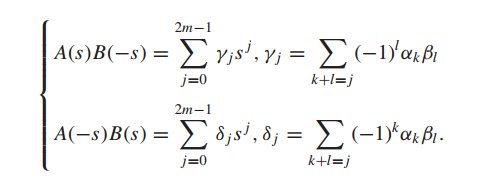
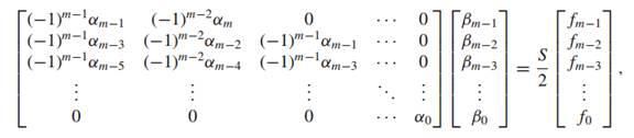
假设多项式:
那么:
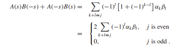
并且满足
记SN(s)N(-s)=
自动校正函数可以通过下式计算:
|
咨询电话
0371-68632068