Data Interpolation and Statistical Analysis(数据插值与统计分析)
3.7.1 Interpolation of One-dimensional Data
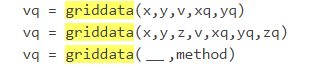
vq
= interp1(x,v,xq,method,extrapolation)
其中x为样品数据,v为对应的样品值,xq为查询点,method为插值方法, extrapolation为外推策略.vq为插值结果.常见的插值方法有’linear’,’nearest’,’next’,’previous’,’pchip’,’cubic’,’v5cubic’,’spline’函数的连续度是不一样的.
[p,S,mu]
= polyfit(x,y,n)
用来对数据开展多项式拟合,其中n为拟合阶数,p为拟合系数,S为误差估计结构体,mu为中值和边界值
Example 3.51 Assume
that the sample points can be generated from a known function
f (x) = (x 2 - 3x + 5)e^-5x sin x, with the following statements. The sample
points generated are
shown in Fig. 3.18(a).(利用既有函数模拟)
3.7.2 Interpolation of Two-dimensional Data

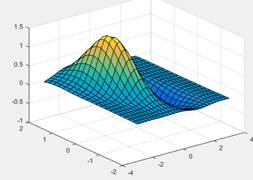
Example 3.52 Consider again the function  given in
Example 2.21. Assume that the sample points are generated in mesh grid form, as
shown in
Fig. 3.20(a). It can be seen that the linear interpolation surface, as the
default form shown in Fig.
3.20(a), is not smooth.在区间[-2 2 ],[-3 3]散点然后插值
数据准备
>> [X,Y]=meshgrid(-2:.5:2,-3:.5:3);
>> Z=(X.^2-2*X).*exp(-X.^2-Y.^2-X.*Y);
>> surf(X,Y,Z)
准备被插值数据,并进行插值计算
>> [X,Y]=meshgrid(-2:.5:2,-3:.5:3);
>> Z=(X.^2-2*X).*exp(-X.^2-Y.^2-X.*Y);
>> surf(X,Y,Z)
>> [x1,y1]=meshgrid(-2:.2:2,-3:.2:3);
>> z1=interp2(X,Y,Z,x1,y1);
>> mesh(x1,y1,z1)

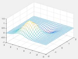
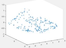
Example 3.53 Consider
the prototype function z = f (x, y) = (x 2 - 2x)e-x2-y2-xy. A set
of sample points (xi, yi) is generated randomly in the
rectangular domain of x ∈ [-3, 3] and
y ∈ [-2, 2].
The distribution of the samples is shown in Fig. 3.21(a). It can be seen that
the
sample points are fairly well distributed. The function values zi can be calculated directly.
With the
griddata() function,
interpolation can be made and interpolation error is assessed.
Girddata具有类似的功能,只是可以指定方法.
x=-3+6*rand(200,1);
y=-2+4*rand(200,1);
z=(x.^2-2*x).*exp(-x.^2-y.^2-x.*y);
mesh(x,y,z)
错误使用 mesh
(line 83)
Z 必须为矩阵,不能是标量或矢量。
%mesh函数不能再用
plot3(x,y,z)
plot3(x,y,z,'x')
%被查数据准备
[x1,y1]=meshgrid(-3:.2:3,-2:.2:2);
z1=interp2(x,y,z,x1,y1);
错误使用 griddedInterpolant
网格矢量必须严格单调递增。
出错 interp2>makegriddedinterp (line 229)
F = griddedInterpolant(varargin{:});
出错 interp2
(line 129)
F =
makegriddedinterp({X, Y}, V,
method,extrap);
%不能使用,必须使用griddata来处理
z2=griddata(x,y,z,x1,y1,'v4');
surf(x1,y1,z2)
3.7.3 Least Squares Curve Fitting
假定xi,yi,i=1,2,3…N被测量,且直到x与y满足函数原型 a是未知量.最小二乘法
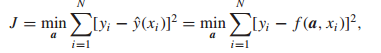
就是用来求解a在什么时候J函数具有最小值

其中Fun是原型函数,a0初始值,x,y为测量数据,am,aM分别为a的边界值,OPT为选项,p为外挂参数
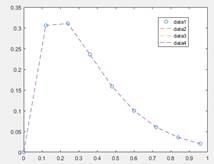
Example 3.54 Consider
the following statements used to generate a set of sample points x
and y
数据生成(模拟测量数据)
x=0:.1:10; y=0.12*exp(-0.213*x)+0.54*exp(-0.17*x).*sin(1.23*x);
假定原型函数为:
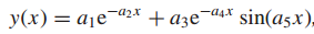 那么
那么
>> x=0:.1:10;
y=0.12*exp(-0.213*x)+0.54*exp(-0.17*x).*sin(1.23*x);
>>
f=@(a,x)a(1)*exp(-a(2)*x)+a(3)*exp(-a(4)*x).*sin(a(5)*x);
[a,e]=lsqcurvefit(f,[1,1,1,1,1],x,y)
即可求得5个待测参数a
3.7.4 Data Sorting
分类函数
[B,I]=sort(A,dim,direction)
Dim是搜索方向 1是行扫描,2为列扫描
Dir是排序方向'ascend' or 'descend'
B为返回向量,I为原始位置
3.7.5 Fast Fourier Transform
对于离散数据xi,是DSP的基础,离散傅里叶变化的表达式为:
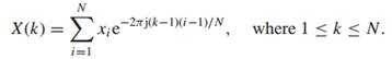
对应的反变化为:
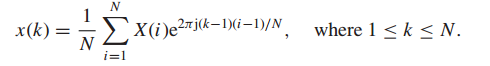
在实践中更为常用的事fft,其效率更高,且不需要2^n-1的约束
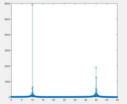
Example 3.55 Assume that the mathematical function is
x(t) = 12 sin(2π × 10t + π/4) + 5 cos(2π × 40t).
Selecting a step size h = 0.01, a set of L time instances ti can be generated. The function
values xi
can be obtained. The corresponding frequencies f0 = 1/(htf), 2 f0, 3 f0,·
· · can be composed, where
tf is the terminating time. The
following statements can be used to draw the relationship between
frequency and magnitude, as shown in Fig. 3.23(a).
>> h=0.01; tf=10; t=0:h:tf;
x=12*sin(2*pi*10*t+pi/4)+5*cos(2*pi*40*t);
>> plot(t,x,'o')
>> X=fft(x);
>> f=t/(h*10);
>> fN=floor(length(f)/2);
>> stem(f(1:fN),abs(X(1:fN)))
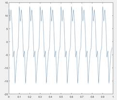
>> ix=real(ifft(X));
>> ii=1:100;
>> plot(t(ii),x(ii),t(ii),ix(ii),':')